Example 9

Case-Study IX: Rainfall-runoff model with spectral likelihood function

Calibration of hydrological models in ungauged basins is the subject of increasing attention by the scientific community. In fact, this is one of the main goals of the Prediction in Ungauged Basins (PUB) initiative promoted by the International Association of Hydrological Sciences (Sivapalan et al., 2003). The present study uses the spectral likelihood function of Whittle (1953) to derive the posterior distribution of the parameters of a hydrologic model. This estimator has good statistical properties, is asymptotically consistent, and has significant advantages over traditional goodness-of-fit criteria in that calibration can be carried out, in principle, with information available in poorly gauged basins. Unlike most statistical estimators that act on the residuals of the observed and simulated data, Whittle’s estimator tries to match the spectral densities of the model output and observed data.

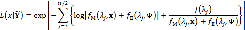
Whittle’s likelihood function is given by

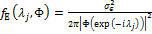
where n is the number of calibration data measurements, are the Fourier frequencies, J is the periodogram (an estimate of the spectral density) of the n-vector of observations, is the spectral density of the simulated discharge time series of the hmodel (depends on the parameter values stored in d-vector x) and is the spectral density of the autoregressive operator , which is equivalent to

where is the standard deviation of the residual vector, between the observed, and simulated, 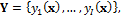discharge record, , and |·| denotes the modulus operator (absolute value).

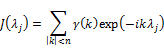
The periodogram of some time series at the frequency can be computed as follows (Brockwell and Davis, 1987)

where is the sample autocovariance coefficient at lag k and i is the imaginary unit. A detailed derivation of Equation (9.01) appears in Whittle (1953) and Beran (1994) provides further analysis of how the spectral likelihood relates to a Gaussian likelihood. Interested readers are referred to these publications for further details.

We now apply Whittle’s estimator to the calibration of a mildly complex lumped watershed model using historical data from the Guadalupe River at Spring Branch, Texas. This is the driest of the 12 MOPEX basins described in the study of Duan et al. (2006). The model structure and hydrologic process representations are found in Schoups and Vrugt (2010). The model transforms rainfall into runoff at the watershed outlet using explicit process descriptions of interception, throughfall, evaporation, runoff generation, percolation, and surface and subsurface routing (see Figure 9.01).

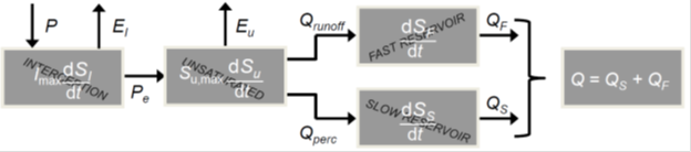
Figure 9.01. Schematic representation of the hmodel conceptual watershed model

Table 9.01 summarizes the seven different model parameters, and their prior uncertainty ranges. These parameters represent conceptual properties of the watershed under investigation, and cannot be measured directly in the field. We therefore derive their values by calibration of the hmodel against a historical record of discharge data.

Table 9.01: Parameters of the hmodel and their prior uncertainty ranges

We use daily discharge, mean areal precipitation, and mean areal potential evapotranspiration from the French Broad watershed at Asheville, North Carolina. We assume herein a multivariate uniform prior distribution for the parameters with ranges listed in Table 9.01. With the use of such flat prior, the posterior density (product of prior and likelihood) is simply proportional to the spectral likelihood function of Equation (9.01). The initial state of each of the N = 10 chains of DREAM is generated with Latin hypercube sampling by drawing from the uniform prior parameter distribution. Standard settings are used for the algorithmic variables.

Implementation of plugin functions

The complete source code can be found in DREAM SDK - Examples\D3\Drm_Example09\Plugin\Src_Cpp