Case-Study XIX: Bayesian Model Averaging: Ensemble Forecasting

Predictive uncertainty analyses is typically carried out using a single conceptual mathematical model of the system of interest, rejecting a priori valid 4 alternative plausible models and possibly underestimating uncertainty in the model itself (Raftery et al., 1999; Hoeting et al., 1999; Neuman, 2003; Raftery et al., 1999; Vrugt et al., 2006, Vrugt and Diks, 2010). Model averaging is a statistical methodology that is frequently utilized in the statistical and meteorological literature to account explicitly for conceptual model uncertainty. The motivating idea behind model averaging is that, with various competing models at hand, each having its own strengths and weaknesses, it should be possible to combine the individual model forecasts into a single new forecast that, up to one’s favorite standard, is at least as good as any of the individual forecasts. As usual in statistical model building, the aim is to use the available information efficiently, and to construct a predictive model with the right balance between model flexibility and overfitting. Viewed as such, model averaging is a natural generalization of the more traditional aim of model selection. Indeed, the model averaging literature has its roots in the model selection literature, which continues to be a very active area of research.

Figure 19.01 provides a simple overview of model averaging. Consider that at a given time we have available the output of multiple different models (calibrated or not). Now the goal is to weight the different models in such a way that the weighted estimate (model) is a better (point) predictor of the observed system behavior (data) than any of the individual models. What is more, the density of the averaged model is hopefully a good estimator of the total predictive uncertainty.

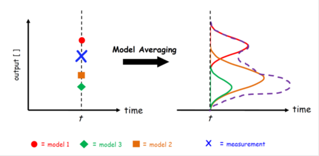
Figure 19.01. Schematic illustration of model averaging using a three member ensemble and single prediction of interest. The forecast of each models are displayed with the solid red circle, blue square and green diamond, respectively, and the verifying observation is indicated separately with the brown “x” symbol. The dotted black line connected with the symbol “o" denotes the weighted average of the forecasts of the three different models. This point predictor satisfies the underlying premise of model averaging as it is in better agreement with the data (smaller distance) than any of the three models of the ensemble. Some model averaging methods also construct a predictive density of this averaged forecast. This overall forecast pdf (solid black line) can be used for probabilistic forecasting and uncertainty analysis, and is simply a weighted average of each ensemble member's predictive distribution (indicated with solid red, blue and green lines) centered at their respective forecasts

To formalize the various model averaging strategies considered herein, let us denote by a vector of measurements of a certain quantity of interest. Further assume that there is an ensemble of K different models available with associated point forecasts 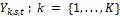at one or more locations s and time, t. If we merge the different model forecasts in a n × K matrix Y (each model has its own column), we can combine their individual forecasts using weighted averaging

where is the jth row of matrix Y which stores the forecasts of each of the K models at a given location and time, is a vector that stores the weights of each individual model, the symbol T denotes transpose, and is a white noise sequence, which will be assumed to have a normal distribution with zero mean and unknown variance.

will often suffice to derive the bias-corrected forecasts, for each of the models of the ensemble. The coefficients and for each of the models, are found by ordinary least squares using the simple regression model

and the observations in the calibration data set. Typically this bias correction leads to a small improvement of the predictive performance of the individual models, with close to zero and close to 1. If the calibration set has relatively few observations, the ordinary least squares estimates become unstable, and bias correction may distort the ensemble (Vrugt and Robinson, 2007). Although a (linear) bias correction is recommended for each of the constituent models of the ensemble, such correction is not made explicit in subsequent notation. For convenience, we simply continue to use the notation rather than for the bias corrected predictors of .

The point forecasts associated with model (19.01) are

where the superscript “e” is used to indicate the expected (predicted) value of the averaged model.

Ensemble Bayesian Model Averaging (BMA) proposed by Raftery et al. (2005) is one popular method for model averaging that is widely used method for statistical post-processing of forecasts from an ensemble of different models. The BMA predictive distribution of any future quantity of interest is a weighted average of probability density functions centered on the bias-corrected forecasts from a set of individual models. The weights are the estimated posterior model probabilities, representing each model's relative forecast skill in the training (calibration) period.

Depending on the type of application one has in mind, different flavors of BMA can be used. For instance, it makes a crucial difference whether one would like to average point forecasts (in which case some forecasts may be assigned negative weights) or density forecasts (in which negative weights could lead to negative forecast densities). We now describe the most popular BMA method which is particularly useful when dealing with the output of dynamic simulation models.

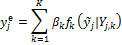
In BMA, each ensemble member forecast, , is associated with a conditional PDF, , which can be interpreted as the conditional PDF of on , given that is the best forecast in the ensemble. If we assume a conditional density, , that is centered on the forecasts of each of the individual models of the ensemble, we can derive the combined forecast density as follows (see also right-hand-side of Figure 19.01)

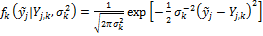
A popular choice for is a normal distribution with mean and variance,

and thus the BMA predictive density, , consists of a mixture of normal distributions, each centered around their individual point forecast . To ensure that represents a proper density, the BMA weights are assumed to lie on the unit simplex, . Thus, the ‘s are nonnegative and add up to one

and they can be viewed as weights reflecting an individual model’s relative contribution to predictive skill over the training (calibration) period.

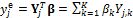
The BMA point predictor is simply a weighted average of the individual models of the ensemble

which is a deterministic forecast in its own way, whose predictive performance can be compared with the individual forecasts in the ensemble, or with the ensemble mean. The associated variance of Equation (19.08) can be computed as (Raftery et al. 2005)

The variance of the BMA prediction defined in Equation (19.08) consists of two terms, the first representing the ensemble spread, and the second representing the within-ensemble forecast variance.

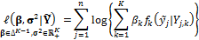
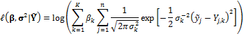
Successful implementation of the BMA method described in the previous section requires estimates of the weights and variances of the PDFs of the individual forecasts. Following Raftery et al. (2005), we use the following formulation of the log-likelihood function, to estimate the values of and in the BMA model

where n denotes the total number of measurements in the training data set. This formulation builds on the assumption that the forecasts errors of the models are independent in space and time. Note, for reasons of numerical stability we work with the log-likelihood function rather than the likelihood function itself. In the case of a normal conditional pdf for the formulation of Equation (19.10) is equivalent to

with and .

Unfortunately, no analytical solutions exist that conveniently maximize Equation (19.10). We therefore use DREAM to derive the posterior distribution of the BMA weights and variances.

In this nineteenth study we apply the BMA method using 48-h forecasts of surface temperature and sea level pressure in the Pacific Northwest in January - June 2000 using the University of Washington (UW) mesoscale short-range ensemble system. This is a five member multianalysis ensemble (hereafter referred to as the UW ensemble) consisting of different runs of the fifth-generation Pennsylvania State University - National Center for Atmospheric Research Mesoscale Model (MM5), in which initial conditions are taken from different operational centers. We assume that all models have a common BMA variance – and thus – which involves inference of parameters with DREAM.  Note, we estimate the standard deviation of the normal predictive pdf, rather than its variance, as this has the advantage of requiring a smaller search space.

A uniform prior distribution is assumed for the BMA weights and variance, and . The initial states of the chains are derived by sampling from the prior distribution of and default values are assumed for the other algorithmic variables.

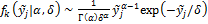
Note, the BMA method of Raftery et al. (2005) was developed for weather quantities such as temperature and sea-level pressure whose conditional pdfs are well described with a normal distribution. The DREAM solver also implements other conditional pdfs that might be more appropriate if the data is skewed. This includes the gamma distribution which much better describes data with a skew

where is a shape parameter, and denotes a scale parameter. These two values depend on the value of but this is beyond of the present case study. Interested readers are referred to Vrugt and Robinson (2007) for an explanation and treatment of three different conditional pdfs. This includes also treatment of heteroscedasticity in the choice of the BMA variance (variance dependent on magnitude of model forecast).

Implementation of plugin functions

The complete source code can be found in DREAM SDK - Examples\D3\Drm_Example19\Plugin\Src_Cpp