Example 18

Case-Study XVIII: Lotka-Volterra: The use of informal likelihoods

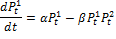
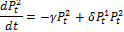
The eighteenth case study reports on GLUE and involves application of an informal likelihood function to the study of animal population dynamics. One of the first models to explain the interactions between predators and prey was proposed in 1925 by the American biophysicist Alfred Lotka and the Italian mathematician Vito Volterra. This model, one of the earliest in theoretical ecology, has been widely used to study population dynamics, and is given by the following system of two coupled differential equations

where and denote the size of the prey and predator population at time t respectively, (-) is the prey growth rate (assumed exponential in the absence of any predators), (-) signifies the attack rate (prey mortality rate for per-capita predation), (-) represents the exponential death rate for predators in the absence of any prey, and (-) is the efficiency of conversion from prey to predator.

A synthetic monthly data set of a prey and predator population is created by solving Equation (18.01) numerically for a 20-year period using an implicit, time-variable, integration method. The initial states, and and parameter values , , and correspond to data collected by the Hudson Bay Company between 1900 and 1920. These synthetic monthly observations are subsequently perturbed with a homoscedastic error, and this corrupted data set is stored in the n-vector and used for inference with DREAM. We now use this data set of “observed” predator and prey abundances to determine the posterior parameter distribution of the four Lotka-Volettera model parameters, hence the parameter vector, .

Table 18.01: Parameters of the Lotka Volterra model in Equation (18.01)

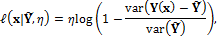
A uniform prior parameter distribution is assumed using the ranges listed in Table 18.01. The initial states of each of the N = 10 Markov chains in DREAM are sampled randomly from the prior ranges using Latin hypercube sampling. An informal GLUE-type likelihood function is used to determine the behavioral (= posterior) solution space. The log-likelihood, is given by

where is a GLUE-coefficient which determines the peakedness of the likelihood surface, and the operator computes the variance of the error residuals between the simulated and observed data (numerator) and variance of the measurement data (denominator), respectively. We assume a value of and use default values of the algorithmic variables of DREAM.

Implementation of plugin functions

The complete source code can be found in DREAM SDK - Examples\D3\Drm_Example18\Plugin\Src_Cpp