Case-Study XVI: Hydrogeophysics: Inference of the spatial distribution of soil properties
The sixteenth case study considers the application of DREAM to distributed soil moisture estimation using travel-time observations from crosshole ground-penetrating radar experiments. This study differs from most other built-in studies of DREAM suite as it requires two- dimensional numerical simulation and high resolution spatial characterization. Such spatial inference problems can be much harder to solve than problems involving temporal characterization of one or more variables of interest. This all has to do with parameter selection. For temporal inference problems, the calibration parameters are usually unknowns in the underlying (differential) equations of the model. These parameters are easy to isolate. For spatial inference problems, it is not only clear how to describe mathematically or statistically the spatial properties of the variable of interest, but it is also unclear how many parameters to use to characterize the observed pattern.
The parameterization of the inverse model should ideally provide enough details to capture all relevant variations in the Earth’s property field and thereby avoid bias caused by model truncation (Trampert and Snieder, 1996). In global earth seismology, it is widely recognized that differences between deterministic inversion results based on the same data set are largely due to differences in spatial or spectral resolutions used in the (inverse) parameterizations (e.g., Chiao and Kuo, 2001). Compactly supported pixels that in a Cartesian coordinate system would be represented by, for example, uniform grid models, provide a very high spatial resolution, whereas spherical harmonics or discrete cosine transform (DCT) in its Cartesian counterpart provide a high spectral resolution. Many popular model parameterization schemes can be found in-between these two opposing extremes, such as wavelets (e.g., Chiao and Kuo, 2001) and slepian functions (e.g., Simons et al., 2006).
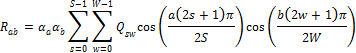
The uniform grid parameterization has the key advantage of a localized and uniform spatial resolution. Inversion based on a uniform grid distribution is hence straightforward. One simply discretizes the spatial domain of interest into a number of cells, and then treats each cell as a different parameter, say, the soil moisture content. This Cartesian parameterization is perhaps straightforward to implement and use, but it is rather inefficient as many thousands of unknowns are required to represent with some spatial resolution and accuracy the soil moisture distribution. This inference problem is unnecessarily difficult and CPU-demanding to solve for DREAM. We therefore use herein a more parsimonious, and perhaps more intelligent, parameterization method and describe the value of the relative saturation (0-100%) of each grid cell using the discrete cosine transform. This transformation, hereafter referred to as the DCT has desirable advantages for stochastic inversion, in that (i) the resolution and separation of scales is explicitly defined, (ii) the transformation is orthogonal and close to the optimal Karhunen-Loève transform, (iii) the computational efficiency is high, (iv) the basis vectors depend only on the dimensionality of the model, and (v) the transformation is linear and operates with real parameter values (Linde and Vrugt, 2013; Qin et al., 2016). The DCT coefficient,  is computed using
|
(16.01) |
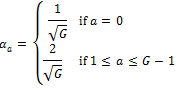
where  and
and  denote the row and column number of the DCT coefficient-matrix, R and the
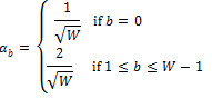
  matrix Q stores a map of discretized values of the relative saturation of the spatial domain of interest and
|
(16.02) |
Close inspection of Equation (16.01) demonstrates that the size of matrix R is exactly similar to that of Q, and thus the standard DCT operation does not reduce parameter dimensionality. Indeed, each coordinate of the matrix Q with value of the soil moisture content, has its own DCT coefficient. We can transform the matrix Q from the space domain to the frequency domain using the DCT coefficients stored in R. The information in this transformation is concentrated in the lower frequencies DCT coefficients. We can thus safely discard the higher frequency DCT coefficients without losing significant information about the spatial pattern of the soil moisture content. The lower frequency DCT coefficients are retained and define the model parameters,  that will be estimated using DREAM. This approach significantly reduces the dimensionality of the parameter space (Linde and Vrugt, 2013; Qin et al., 2016) and has desirable advantages for stochastic inversion.
For example, Figure 1 in Jafarpour et al. (2008) depicts the results for the first 8 × 8 DCT bases and shows how the DCT transform coefficients relate to a given geological model. The more DCT coefficients are used the better the reconstruction of the true field (see Qin et al., 2016). We use herein  DCT coefficients, which jointly maintain about 95-97% of the variance of the original relative saturation space.
As a synthetic example, we use a soil moisture model from Kowalsky et al. (2005). This model was constructed by simulating an infiltration experiment in a heterogeneous soil. The simulated soil moisture distribution is transformed into a radar velocity model using Topp’s equation (Topp et al., 1980) (Fig. 1a). A synthetic data set of 900 travel-time observations is constructed for two different boreholes located 3 m apart using a transmitter-receiver geometry consisting of multiple-offset gathers between 0 and 3 m depth with sources and receiver intervals of 0.1 m. The resulting travel times calculated with the time3d algorithm (Podvin and Lecomte, 1991) are contaminated with zero mean uncorrelated Gaussian noise with a standard deviation of 0.5 nanoseconds, ns. This constitutes a high-quality GPR data set, which is subsequently used to compare our MCMC inversion methodology against exact theory, but with noisy data.
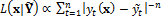
We use a simple Gaussian likelihood function
|
(16.03) |
where  and
and  are the observed and simulate travel-time data respectively, and n denotes the number of measurements. The simulated travel-time data are derived from the DCT coefficients of the relative moisture distribution using a simple linear travel-time simulator. This model is a simplified version of the numerical model used by Linde and Vrugt (2013) as it considers straight rays only. This simplification reduces the CPU-cost of the model tremendously, yet can only provide approximate results.
The initial state of each Markov chain is drawn from  , a normal distribution centered at zero and with covariance matrix equal to
  . All the off-diagonal elements of this matrix are set to zero and the main diagonal contains values of about 0.017 (first element) and 0.05 and 0.07, respectively. These values are deliberately set small so that DREAM needs relatively few iterations to converge to the posterior distribution. We use N = 32 chains with DREAM to generate samples of the posterior distribution of the moisture distribution and use thinning of the chains (each 5th sample is collected) to minimize memory storage. Default settings are assumed for all other algorithmic variables of DREAM.
Implementation of plugin functions
The complete source code can be found in DREAM SDK - Examples\D3\Drm_Example16\Plugin\Src_Cpp