Example 6

Case-Study VI: A conceptual watershed model with generalized log-likelihood function

The sixth case study involves flood forecasting, and consists of the calibration of a mildly complex lumped watershed model using historical data from the Guadalupe River at Spring Branch, Texas. This is the driest of the 12 MOPEX basins described in the study of Duan et al. (2006). The model structure and hydrologic process representations are found in Schoups and Vrugt (2010). The model transforms rainfall into runoff at the watershed outlet using explicit process descriptions of interception, throughfall, evaporation, runoff generation, percolation, and surface and subsurface routing (see Figure 6.01).

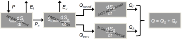
Figure 6.01. Schematic representation of the hmodel conceptual watershed model.

Table 6.01 summarizes the seven different parameters of the hmodel and their prior uncertainty ranges. While some of the values of parameters in conceptual rainfall-runoff models can be derived directly from knowledge of physical watershed characteristics, others are effective quantities that cannot, in practice, be measured in the field, and therefore have to be estimated through calibration against a measured streamflow hydrograph using either a trial-and-error ‘manual approach’ or an automated search algorithm (Boyle et al., 2000; Madsen, 2000). The parameters, which are estimated in this manner, represent effective conceptual representations of spatially and temporally heterogeneous watershed properties. A model calibrated by such means can be used for the simulation or prediction of hydrologic events outside of the historical record used for model calibration, if it can be reasonably assumed that the physical characteristics of the watershed and the hydrologic/climate conditions remain similar (Gupta et al., 2002; Vrugt et al., 2006).

Table 6.01: Parameters of the hmodel and their prior uncertainty ranges

We calibrate the parameters of hmodel using daily discharge, mean areal precipitation, and mean areal potential evapotranspiration from the French Broad watershed at Asheville, North Carolina. We assume a multivariate uniform prior distribution for all seven model parameters using the ranges listed in Table 6.01.

An assumption made in many studies published in the literature is that the residuals between modeled and observed discharge data are normally distributed. This then leads to a standard Gaussian likelihood function (see previous two studies).  We deviate from this assumption in this case study and use instead the generalized likelihood function developed by Schoups and Vrugt (2010) which extends the applicability of previously used likelihood functions to situations where residual errors are correlated, heteroscedastic, and non-Gaussian with varying degrees of kurtosis and skewness. The approach focuses on a correct statistical description of the data and the total model residuals, without separating out various error sources. The generalized likelihood function is given by

       (6.01)

where is a n-vector with observed discharge data, n denotes the number of measurements, is the estimated measurement error of the discharge data, 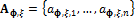is a n-vector of filtered error residuals using an autoregressive model with coefficients, , and , , and are computed as function of the skewness parameter, , and kurtosis parameter, , and |·| denotes the modulus operator (absolute value). The scalars 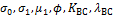are so called nuisance variables whose values are either fixed or estimated jointly with the model parameters. These nuisance variables are discussed in Table 6.02 below. The discharge measurement error is computed using where 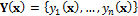is the hmodel simulated record of discharge values using the values of the model parameters and nuisance variables stored in the d-vector x.

† The listed units and ranges depend on units and characteristics of calibration data (discharge in present case)

Table 6.02: Nuisance variables of the generalized log-likelihood function†

The nuisance variables that are highlighted in blue are estimated along with the parameters of the hmodel. Their prior distribution is assumed uniform using the ranges listed above. The other nuisance variables in the generalized likelihood function of Equation (6.01) are set to their default values. This equates in a total of 11 parameters whose posterior distribution needs to be sampled with DREAM by calibration of the hmodel against the observed discharge data of the French Broad River. The initial population of the model parameters and nuisance variables is drawn from the lower and upper ranges listed in Table 6.01 and 6.02 using Latin hypercube sampling. We use N = 11 chains with DREAM to generate samples from the posterior parameter distribution using standard settings for the algorithmic variables.

Implementation of plugin functions

The complete source code can be found in DREAM SDK - Examples\D3\Drm_Example06\Plugin\Src_Cpp