Example 23

Case-Study XXIII: Limits of Acceptability: The SAC-SMA flood forecasting model

The twenty-third case study involves the modeling of the rainfall-runoff transformation of the Leaf River watershed in Mississippi. This temperate 1944 km2 watershed has been studied extensively in the hydrologic literature which simplifies comparative analysis of the results. The rainfall-discharge relationship of the Leaf River basin is simulated using the Sacramento soil moisture accounting (SAC-SMA) model of Burnash (1973). This lumped conceptual watershed model is used by the National Weather Service for flood forecasting through the United States. The SAC-SMA model uses six reservoirs (state variables) to represent the rainfall-runoff transformation. These reservoirs represent the upper and lower part of the soil and are filled with "tension" and "free" water, respectively. The upper zone simulates processes such as direct runoff, surface runoff, and interflow, whereas the lower zone is used to mimic groundwater storage and the baseflow component of the hydrograph.

Figure 23.01 provides a schematic overview of the SAC-SMA model. Nonlinear equations are used to relate the absolute and relative storages of water within each reservoir and their states control the main watershed hydrologic processes such as the partitioning of precipitation into overland flow, surface runoff, direct runoff, infiltration to the upper zone, interflow, percolation to the lower zone, and primary and supplemental baseflow. Saturation excess overland flow occurs when the upper zone is fully saturated and the rainfall rate exceeds interflow and percolation capacities. Percolation from the upper to the lower layer is controlled by a nonlinear process that depends on the storage in both soil zones.

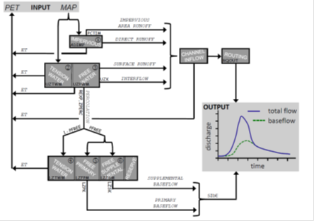
Figure 23.01. Schematic representation of the Sacramento soil moisture accounting (SAC-SMA) conceptual watershed model. The parameters of the SAC-SMA model appear in Comic Sans font type (black), whereas Courier font type is used to denote the individual fluxes computed by the model. Numbers are used to denote the different SAC-SMA state variables, (1) ADIMC, (2) UZTWC, (3) UZFWC, (4) LZTWC, (5) LZFPC, and (6) LZFSC. The ratio of deep recharge to channel base ow (SIDE) and other remaining SAC-SMA parameters RIVA and RSERV are set to their default values of 0.0, 0.0 and 0.3, respectively

The SAC-SMA model has thirteen user-specifiable (and three fixed) parameters and an evapotranspiration demand curve (or adjustment curve). Inputs to the model include mean areal precipitation (MAP) and potential evapotranspiration (PET) while the outputs are estimated evapotranspiration and channel inflow. A unit hydrograph or kinematic wave routing model is often used to rout channel inflow downstream to the gauging point. Here, I use instead a Nash-Cascade series of three linear reservoirs to rout the upper zone channel inflow whereas the baseflow generated by the lower zone recession is passed directly to the gauging point. This configuration adds one parameter and three state variables to the SAC-SMA model. The use of the three reservoirs improves considerably the CPU-efficiency as it avoids the need for computationally expensive convolution. Our formulation of the model therefore has fourteen time-invariant parameters which are subject to inference using observed discharge data. Table 23.01 summarizes the fourteen SAC-SMA parameters and their prior uncertainty ranges. We also list the six main state variables.

Table 23.01: Parameters of the SAC-SMA model and their prior uncertainty ranges

In the manifesto for the equifinality thesis, Beven (2006) suggested that a more rigorous approach to model evaluation would involve the use of limits of acceptability for each individual observation against which model simulated values are compared. Within this framework, behavioral models are defined as those that satisfy the limits of acceptability for each observation. Ideally, the limits of acceptability should reflect the observational error of the variable being compared, together with the effects of input error and commensurability errors resulting from time or space scale differences between observed and predicted values Beven (2014). The limits of acceptability approach has been used by various authors (Blazkova and Beven, 2009; Dean et al., 2009; Krueger et al., 2009; Liu et al., 2009; Mcmillan et al., 2010; Westerberg et al., 2011), although earlier publications used similar ideas within GLUE based on fuzzy measures (Page et al., 2003; Freer et al.,2004; Page et al., 2004, 2007, Pappenberger et al., 2005, 2007). The limits of acceptability framework might be considered more objective than the standard GLUE approach advocated in Beven (1992) as the limits are defined before running the model on the basis of best available hydrologic knowledge.

In this study we apply the limits of acceptability approach to the SAC-SMA model using data from the Leaf River watershed in the USA. A 10-year historical record (1/10/1952 - 30/9/1962) with daily data of discharge (mm/day), mean areal precipitation (mm/day), and mean areal potential evapotranspiration (mm/day) is used herein for SAC-SMA model calibration. A 65-day spin-up period is used to reduce sensitivity of the model to state-value initialization. We store the daily discharge observations in the n-vector, .

We are now left with definition of the effective observation error (limits of acceptability) of each discharge observation. This error varies dynamically with flow level and constitutes the combined effect of input data, model structural and calibration data measurement error. Here, we follow the approach of Sadegh and Vrugt (2013) and define the limits of acceptability as a multiple of the actual discharge measurement error. I follow Vrugt et al. (2005) and use a nonparametric estimator to calculate the measurement data error of the n discharge observations, hereafter referred to as . The limits of acceptability are now computed as multiple of or using . This leads to effective observation errors on the order of . The following pseudo-likelihood function is used to determine the goodness-of-fit of each simulated discharge record

where is an indicator function that returns one if the condition a is satisfied and zero otherwise. Parameter values whose SAC-SMA simulation leads to a score of Equation (23.01) equal to , honor the limits of acceptability of each discharge observation, and are called behavioral solutions.

We now explore the behavioral solution space (might not exist!) with DREAM. We assume a uniform prior parameter distribution using the ranges listed in Table 23.01 and draw the initial position of the different Markov chains using Latin hypercube sampling. Default values of the algorithmic variables are used.

Implementation of plugin functions

The complete source code can be found in DREAM SDK - Examples\D3\Drm_Example23\Plugin\Src_Cpp