Case-Study XII: Pedometrics (variogram fitting)

The past decades have seen a growing interest in soil characterization, not only because many highly interrelated water, carbon, and vegetation processes take place in this part of our ecosystem, but also because the subsurface plays a major role in carbon storage, exchange of water and soil vapor with the ambient atmosphere, and contaminant transport to the groundwater. Many soil properties not only exhibit significant spatial and temporal variability, but are also difficult to measure directly. Geostatistics is primarily concerned with the mathematical description, prediction, and uncertainty analysis of these spatially varying variables.

The basis of geostatistical estimation is the assumption that an observation of a variable at location s is a realization of a random field . The random function is assumed to be intrinsically stationary (Webster and Oliver, 2009)

and

where h is a lag vector, and γ(h) is the variogram. The method of moments is usually used to estimate the so-called empirical variogram, and parameters of a variogram model are then estimated by fitting a model to the empirical variogram. Thus, the accuracy of spatial prediction is determined by how the variogram is estimated.

The paper of Diggle et al. (1998) introduced an alternative approach to geostatistical inference that is based on the application of formal statistical methods. This so-called model-based Geostatistics relies on general principles of statistical inference and use an explicit stochastic error model of the data. The use of a proper likelihood function and a posteriori check of the error residual distribution not only constitutes good statistical practice, but also facilitates the application of a powerful array of multivariate statistical analyses to explore the marginal and joint posterior probability density functions of the nugget, sill and range. Other formal statistical approaches include the generalized linear-mixed model and empirical best linear unbiased prediction (EBLUP) (Zimmerman and Cressie, 1992). Despite this progress made, it remains typically difficult to estimate the parameters of a variogram model and successfully solve the geostatistical inverse problem. That is, the covariance structure of the residuals is required for variogram fitting, yet in most cases is unknown a priori. The spatial covariance structure can only be obtained after fitting the trend. The residual maximum likelihood (REML) approach is therefore advocated (Lark et al., 2006), because it allows for independent estimation of the covariance structure by transforming the data into stationary increments that filtered out the trend. Nevertheless, REML or related methods only attempt to find the maximum likelihood values of the variogram parameters without recourse to estimating their underlying posterior uncertainty. This posterior probability distribution function (pdf) contains important information about the uncertainty and correlation of the various geostatistical parameters and can be used to derive meaningful estimates of spatial prediction uncertainty.

In this twelfth case study we explore the use of Markov chain Monte Carlo simulation with DREAM to characterize the uncertainty of the variogram parameters and their effect on spatial prediction uncertainty.

We assume herein a simple linear trend model for prediction of variable y at n different locations . This model can be written as

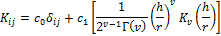
where , signifies a matrix with spatial coordinates, is the design matrix of the trend function , is a vector of trend parameters, and is the vector of residuals with a mean of zero and covariance matrix, K. This covariance can be described with the Matérn function

where Kij is the covariance between observation i and j, h represents the separation distance between i and j, denotes the Kronecker delta (= 1 if i = j and = 0 when i ≠ j), c0 is the nugget variance, and c0 + c1 signifies the sill variance, Kν is a modified Bessel function of the second kind of order ν, Γ is the gamma function, r denotes the distance or ‘range’ parameter and ν is the “smoothness”. This latter parameter allows for great flexibility in modelling of the local spatial covariance. The Matérn function is equivalent to the exponential function for , the Whittle model (1954) for and approaches the Gaussian model for . 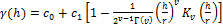The corresponding semivariance of the Matérn function is

The parameters of this function can be summarized in a single vector, .

The value of at the unsampled location can be computed from

where are the observed values at each of the n measurement locations, M is the design matrix , , and . The associated variance of the prediction at location is

where and .The unknown parameters in Equations (12.06) – (12.07) are now combined in the vector, and estimated using Markov chain Monte Carlo simulation with DREAM. This allows for characterization of the uncertainty of the trend and variogram parameters and their effect on spatial prediction uncertainty.

We use herein a single trend parameter for (also referred to as “mean”), thus resulting in a -dimensional parameter estimation problem. Table 12.01 summarizes the trend and variogram parameters which are subject to inference and their prior uncertainty ranges.

† Listed units and ranges depend on units and characteristics of calibration data

Table 12.01: Trend and variogram parameters and their prior uncertainty ranges

We use soil thickness data of the A horizon collected at an experimental field plot near Forbes, New South Wales, Australia (Pettitt and McBratney, 1993). A nested sampling design was used where the field was divided into 18 equal-sized blocks of 160 m2. In each block six sampling points were used along transects of 156 m long separated by 125 m, 25 m, 5 m, 1 m and 25 cm.

To successfully implement DREAM we need to define the parameter ranges, an initial sampling distribution, and a likelihood function to compare the model predicted A-thickness with the observed data. In this case study, we assume a uniform prior distribution with upper and lower bounds of the parameters listed in Table 12.01, and use Latin Hypercube sampling over this d-dimensional hypercube to initialize the starting points of the N = 10 different Markov chains. The following formulation of the log-likelihood function, is used (Mardia and Marshall, 1984)

where is the covariance matrix derived from the Matérn function, signifies the determinant operator, and is a scalar whose value does not affect the posterior parameter distribution. This latter value is therefore ignored. We assume default values for the algorithmic variables of DREAM.

Implementation of plugin functions

The complete source code can be found in DREAM SDK - Examples\D3\Drm_Example12\Plugin\Src_Cpp